Tidyverse Other packages

Dr. Md. Zulquar Nain

tidyr - Data Tidying

A package in the Tidyverse for tidying data
Helps convert data between wide and long formats
Simplifies reshaping and cleaning datasets
Key Functions in tidyr

pivot_longer()

Converting from Wide data (multiple columns for the same variable) to Long data (one column for each variable)

library(tidyr)
  
  data_wide <- tibble(
    id = 1:3,
    `2021` = c(100, 150, 200),
    `2022` = c(110, 160, 210)
  )
  
  data_long <- data_wide %>%
    pivot_longer(cols = `2021`:`2022`, names_to = "year", values_to = "value")
  
  print(data_long)

# A tibble: 6 × 3
     id year  value
  <int> <chr> <dbl>
1     1 2021    100
2     1 2022    110
3     2 2021    150
4     2 2022    160
5     3 2021    200
6     3 2022    210

pivot_wider()

Converting from Long to Wide Format

data_long <- tibble(
  id = c(1, 1, 2, 2, 3, 3),
  year = c("2021", "2022", "2021", "2022", "2021", "2022"),
  value = c(100, 110, 150, 160, 200, 210)
)

data_wide <- data_long %>%
  pivot_wider(names_from = year, values_from = value)

print(data_wide)

# A tibble: 3 × 3
     id `2021` `2022`
  <dbl>  <dbl>  <dbl>
1     1    100    110
2     2    150    160
3     3    200    210

separate()

Splits a single column into multiple columns

data <- tibble(name = c("John Doe", "Jane Smith", "Alice Johnson"))

data_separated <- data %>%
  separate(name, into = c("first_name", "last_name"), sep = " ")

print(data_separated)

# A tibble: 3 × 2
  first_name last_name
  <chr>      <chr>    
1 John       Doe      
2 Jane       Smith    
3 Alice      Johnson

unite()

Combines multiple columns into one

data <- tibble(first_name = c("John", "Jane", "Alice"),
               last_name = c("Doe", "Smith", "Johnson"))

data_united <- data %>%
  unite("full_name", first_name, last_name, sep = " ")

print(data_united)

# A tibble: 3 × 1
  full_name    
  <chr>        
1 John Doe     
2 Jane Smith   
3 Alice Johnson

drop_na()

Removes rows with missing values

data <- tibble(x = c(1, NA, 3), y = c(4, 5, NA))

data_clean <- data %>%
  drop_na()

print(data_clean)

# A tibble: 1 × 2
      x     y
  <dbl> <dbl>
1     1     4

fill()

Fills missing values using the previous or next available value

data <- tibble(x = c(1, NA, 3, NA, 5))

data_filled <- data %>%
  fill(x, .direction = "down")

print(data_filled)

# A tibble: 5 × 1
      x
  <dbl>
1     1
2     1
3     3
4     3
5     5

tidyr vs dplyr

tidyr: Specializes in reshaping and tidying data (e.g., pivot_longer(), pivot_wider(), separate()).
dplyr: Specializes in data manipulation, such as subsetting, grouping, and summarizing (e.g., filter(), mutate(), summarize()).

readr - Data Import/Export

part of the tidyverse, focused on reading and writing rectangular data (e.g., CSV, TSV).
Faster and more consistent than base R functions
Makes data handling easy and efficient.
Key Functions:

read_csv()

library(readr)
data_csv <- read_csv("hsbraw.csv")
head(data_csv)

# A tibble: 5 × 1
      x
  <dbl>
1     1
2    NA
3     3
4    NA
5     5

read_delim()

# Read a pipe-separated file
data_pipe <- read_delim("hsbraw.txt", delim = "|")
head(data_pipe)

# A tibble: 5 × 1
      x
  <dbl>
1     1
2    NA
3     3
4    NA
5     5

write_csv()

# Write a data frame to a CSV file
write_csv(data, "hsbraw.csv")

write_delim()

# Write data to a pipe-separated file
write_delim(data, "hsbraw.txt", delim = "|")

purrr - Functional Programming

enhances R’s functional programming capabilities by providing a consistent, simple way to apply functions to lists, vectors, and other data structures.
Key function:-

map()

Applies a function to each element of a list and returns a list.

library(purrr)

# Create a list of numbers
numbers <- list(1, 2, 3, 4, 5)

# Apply a function to square each number using map
squared_numbers <- map(numbers, ~ .x^2)

# Print the result
squared_numbers

[[1]]
[1] 1

[[2]]
[1] 4

[[3]]
[1] 9

[[4]]
[1] 16

[[5]]
[1] 25

map_dbl()

To apply a function and return a vector (not a list), map_dbl() is used.

# Apply the same function, but return a vector of doubles
squared_numbers_vector <- map_dbl(numbers, ~ .x^2)

# Print the result
squared_numbers_vector

[1]  1  4  9 16 25

map2()

Applies a function to two inputs simultaneously.
useful when you need to operate on two lists.

# Create two lists
list1 <- list(1, 2, 3)
list2 <- list(10, 20, 30)

# Use map2 to add corresponding elements
sum_list <- map2(list1, list2, ~ .x + .y)

# Print the result
sum_list

[[1]]
[1] 11

[[2]]
[1] 22

[[3]]
[1] 33

map_chr()

Used to get a character vector instead of a numeric one.

# Create a list of numbers
numbers2 <- list(1, 2, 3, 4)

# Use map_chr to convert each number to a character string
char_numbers <- map_chr(numbers2, ~ as.character(.x))

# Print the result
char_numbers

[1] "1" "2" "3" "4"

purrr vs tidyr

purrr is specifically focused on working with lists and vectors using functional programming techniques.
tidyr is focused on reshaping data frames (long to wide format and vice versa), separating and combining columns.

tibble - Modern Data Frames

A modern version of a data frame.
More robust and user-friendly than traditional data frames.
Improved handling of large data sets

Basic Tibble

# Create a basic tibble
people_tibble <- tibble(
  Name = c("John", "Alice", "Bob"),
  Age = c(25, 30, 22),
  Location = c("New York", "London", "Paris")
)

# Print the tibble
people_tibble

# A tibble: 3 × 3
  Name    Age Location
  <chr> <dbl> <chr>   
1 John     25 New York
2 Alice    30 London  
3 Bob      22 Paris

Tibble with Mixed Data Types

# Create a tibble with mixed data types
mixed_tibble <- tibble(
  Name = c("John", "Alice", "Bob"),
  Age = c(25, 30, 22),
  Is_Active = c(TRUE, FALSE, TRUE),
  Height = c(5.9, 5.6, 6.1)
)

# Print the tibble
mixed_tibble

# A tibble: 3 × 4
  Name    Age Is_Active Height
  <chr> <dbl> <lgl>      <dbl>
1 John     25 TRUE         5.9
2 Alice    30 FALSE        5.6
3 Bob      22 TRUE         6.1

Tibble vs. Data Frame

Data Frame

Displays all rows, which can be overwhelming with large datasets.
Automatically converts character vectors to factors (unless specified otherwise).

Tibble

Only shows the first few rows, making it easier to handle large datasets.
Does not convert character columns into factors by default, avoiding a common issue with data frames.

stringr - String manipulation

Provides simple functions for common text operations.
Focuses on consistency and ease of use.
Key Functions:-

str_detect()

# checks if a pattern exists in the string
library(stringr)
text <- "Hello, world!"
has_hello <- str_detect(text, "Hello")
has_hello

[1] TRUE

str_replace()

#replaces the first occurrence of a pattern with a new string
text <- "I love R programming."
new_text <- str_replace(text, "R", "Python")
new_text

[1] "I love Python programming."

str_replace_all()

# replaces all occurrences of a pattern
text <- "The cat is on the mat. The cat is cute."
new_text_all <- str_replace_all(text, "cat", "dog")
new_text_all

[1] "The dog is on the mat. The dog is cute."

str_sub()

#extracts a substring from a string
text <- "Hello, world!"
substring <- str_sub(text, 1, 5)
substring

[1] "Hello"

str_to_lower()

# converts all characters in the string to lowercase
text <- "HELLO, WORLD!"
lowercase_text <- str_to_lower(text)
lowercase_text

[1] "hello, world!"

str_split()

#splits a string into a list by a specified delimiter 
text <- "apple,banana,cherry"
split_text <- str_split(text, ",")
split_text

[[1]]
[1] "apple"  "banana" "cherry"

str_length()

#returns the number of characters in the string
text <- "Hello"
string_length <- str_length(text)
string_length

[1] 5

lubridate

It makes working with date-times easier
Provides functions to manipulate, parse, and format date-time data.
Simplifies operations like extracting parts of date-time, arithmetic operations, and handling time zones.

Parsing Dates

library(lubridate)
# Parse a date in year-month-day format
date1 <- ymd("2025-03-03")
print(date1)

[1] "2025-03-03"

Parsing Dates with Time

# Parse a date-time with time and time zone
datetime1 <- ymd_hms("2025-03-03 12:30:45")
print(datetime1)

[1] "2025-03-03 12:30:45 UTC"

Extracting Date-Time Components

# Extract components from a date-time object
year(datetime1)

[1] 2025

month(datetime1)

[1] 3

day(datetime1)

[1] 3

hour(datetime1)

[1] 12

minute(datetime1)

[1] 30

second(datetime1)

[1] 45

Handling Time Intervals

# Define an interval
start <- ymd_hms("2025-03-01 00:00:00")
end <- ymd_hms("2025-03-05 23:59:59")
interval1 <- interval(start, end)
print(interval1)

[1] 2025-03-01 UTC--2025-03-05 23:59:59 UTC

forcats - Working with Factors

Makes working with categorical variables easier.
Provides tools to manipulate factors and handle tasks like reordering, renaming, and combining levels.
Key functions :

Creating Factors

library(forcats)
# Create a factor from a vector
categories <- c("Low", "High", "Medium", "Low", "High")
factor_categories <- factor(categories)
print(factor_categories)

[1] Low    High   Medium Low    High  
Levels: High Low Medium

Reordering factor levels

# Reorder factor levels
factor_ordered <- fct_reorder(factor_categories, c(3, 2, 1, 4, 5))
print(factor_ordered)

[1] Low    High   Medium Low    High  
Levels: Medium High Low

Changing Factor Levels

# Change factor levels
new_factor <- fct_recode(factor_categories, "Very Low" = "Low", "Very High" = "High")
print(new_factor)

[1] Very Low  Very High Medium    Very Low  Very High
Levels: Very High Very Low Medium

Combining Factor Levels

# Combine similar factor levels
collapsed_factor <- fct_collapse(factor_categories, 
                                 "Low/Medium" = c("Low", "Medium"),
                                 "High" = "High")
print(collapsed_factor)

[1] Low/Medium High       Low/Medium Low/Medium High      
Levels: High Low/Medium

Working with Factor Levels

# Drop unused factor levels
dropped_factor <- fct_drop(factor_categories)
print(dropped_factor)

[1] Low    High   Medium Low    High  
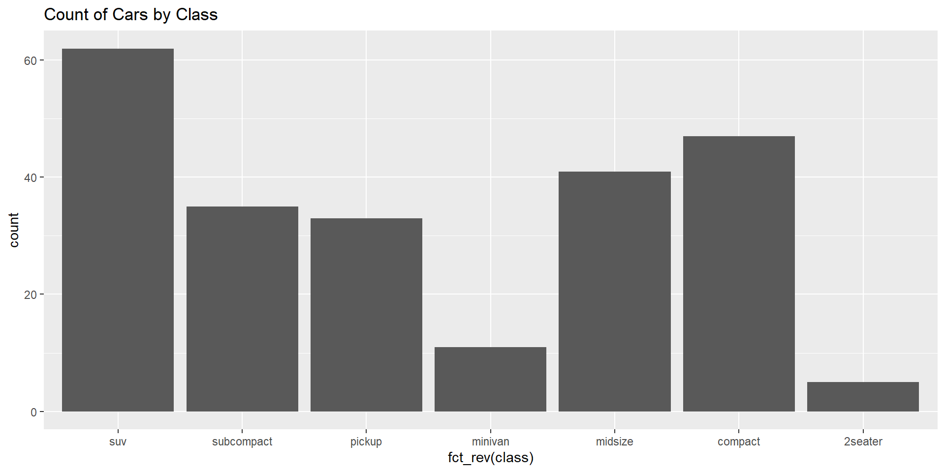
Levels: High Low Medium

Visualizing Factor Data

library(ggplot2)
# Create a plot with reordered factor levels
ggplot(mpg, aes(x = fct_rev(class))) + 
  geom_bar() + 
  labs(title = "Count of Cars by Class")

forcats vs dplyr

forcats works with factors used for modifying factor levels, whereas dplyr also provides some functions that manipulate factors (e.g., mutate() and factor()).
forcats: Designed specifically for working with factors and making factor level manipulations easier.
dplyr: While dplyr can work with factors, forcats is more specialized for factor-specific operations.